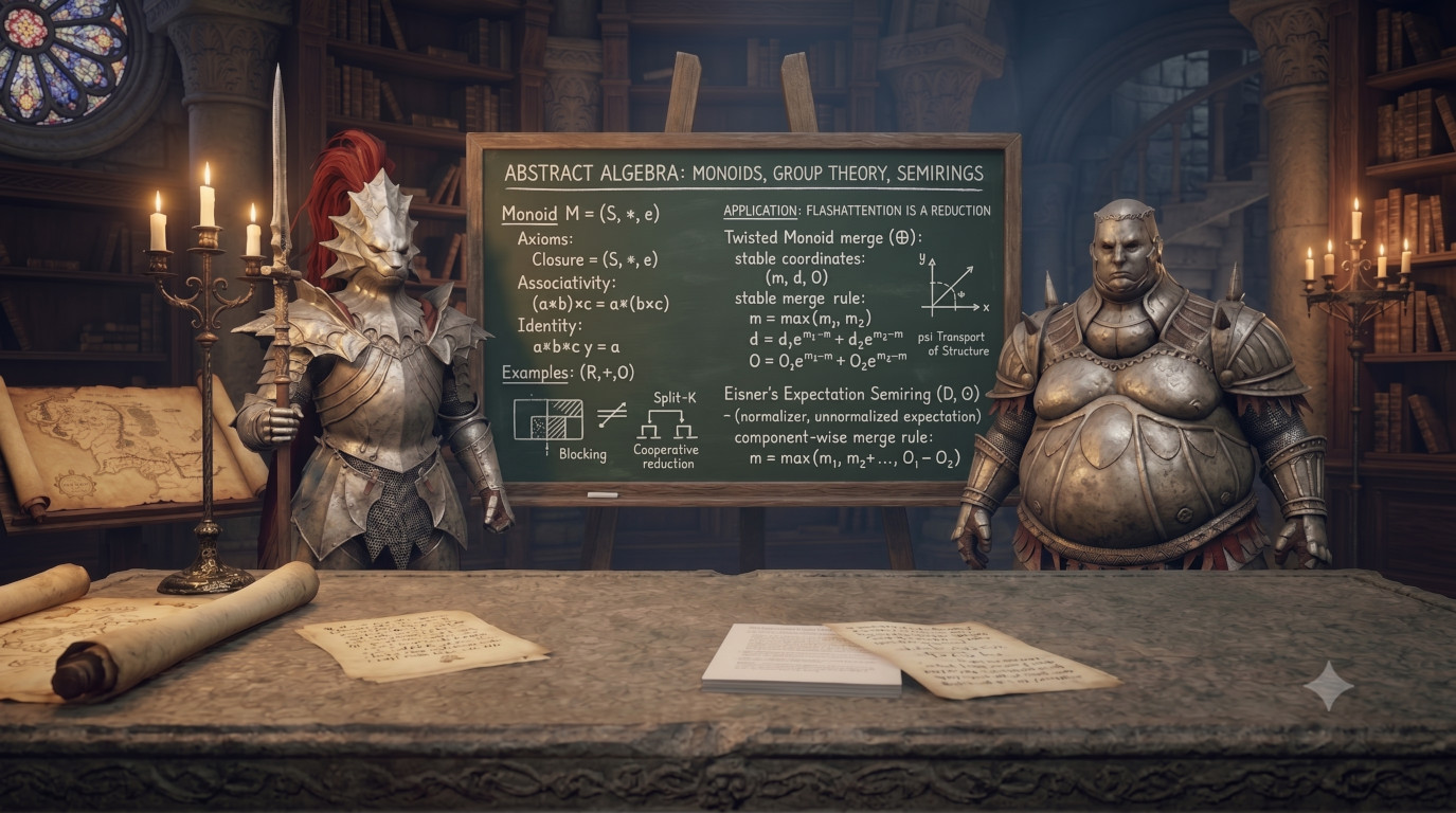
When looking for FlashAttention tutorials online, I was frustrated that existing ones are way too simple! Where's the fun in that? Would you enjoy breezing through a Dark Souls boss on the first attempt? I am here to fix this critical gap and present the Dark Souls of FlashAttention tutorials. Enjoy countless detours into abstract algebra, precision analysis, and other esoteric math exercises.

We've established that you love pain, but is there a point to all these derivations? If you need an extra nudge: the goal is to show that FlashAttention is not a one-of-a-kind deep optimization, but a single example from a much larger class. That matters most if you're interested in how ML compilers work, which must optimize countless models without special-casing.

This is Part 1/2. The theoretical foundation: the algebra that turns attention into an associative reduction, and why that single fact is the only thing its GPU implementation needs. Part 2 (forthcoming) takes this down to the metal and focuses on generating efficient kernels.

Associativity is All You Need

Start with the most boring operation in machine learning: summing a vector.

$$\operatorname{sum}(x) = x_0 + x_1 + \dots + x_{N-1}$$

It is trivially parallelizable, thanks to the associativity of +:

$$(a + b) + c = a + (b + c)$$

Because the bracketing doesn't matter, you can chop the $N$ elements into contiguous chunks, sum each chunk on its own (a thread, a warp, a whole thread block), and then add up the partials:

• Blocking cuts the axis into tiles and sums the tile totals.
• Cooperative reduction gives each thread a strided slice and combines the per-thread partials with a warp shuffle or a shared-memory tree.
• Split-K lets separate thread blocks own chunks, write their partial sums to scratch, and fold them in a small second kernel.

A GPU needs one more thing: a way to deal with the ragged edge. $N$ is almost never a clean multiple of the tile width, and at runtime you might not even know it until the kernel launches. A neutral element lets you mask the overhang: pad the tail with $0$, and one kernel shape stays correct at every length.

Two requirements, then: the operation has to be associative (so chunks split and recombine), and it has to have a neutral element (so tails and masks come for free). An operator with both is a monoid. + with $0$ is one; so are max with $-\infty$, min with $+\infty$, boolean and/or, and matrix-multiply. A compiler that can lower one monoid reduction can therefore lower all of them: only the combine operator changes, never the schedule.

Formally, a monoid is a set $\mathcal{S}$ together with a binary operation $\oplus : \mathcal{S} \times \mathcal{S} \to \mathcal{S}$ and a distinguished element $e \in \mathcal{S}$ satisfying three axioms:

$$\begin{aligned} \textbf{(M1) closure:}\quad & a \oplus b \in \mathcal{S} && \text{for all } a, b \in \mathcal{S} \\ \textbf{(M2) associativity:}\quad & (a \oplus b) \oplus c = a \oplus (b \oplus c) && \text{for all } a, b, c \in \mathcal{S} \\ \textbf{(M3) identity:}\quad & a \oplus e = e \oplus a = a && \text{for all } a \in \mathcal{S} \end{aligned}$$

Softmax Looks Like It Breaks the Rules

Here is the operation we actually want, the softmax of a length-$N$ score vector $s$:

$$\operatorname{softmax}(s)_i = \frac{e^{s_i}}{\sum_{j} e^{s_j}}$$

On paper this is a clean reduction: compute the denominator $\sum_j e^{s_j}$ (a +-monoid over the values $e^{s_j}$), then divide. Floating point spoils the fun. Scores in a transformer routinely climb into the tens, and $e^{90}$ easily overflows float32. So every real implementation reaches for the safe softmax, which subtracts the maximum before exponentiating:

$$m = \max_j s_j \qquad \operatorname{softmax}(s)_i = \frac{e^{s_i - m}}{\sum_{j} e^{s_j - m}}$$

Subtracting $m$ is free (multiply top and bottom by $e^{-m}$), but it rescues the range: every exponent $s_i - m \le 0$, so $e^{s_i - m} \in (0, 1]$ and nothing overflows. The denominator is now $d = \sum_j e^{s_j - m}$.

The catch: $m$ depends on the whole vector, and $d$ depends on $m$. Done naively, that's three passes over $s$. Each pass introduces launch overhead and pays the price of moving elements to and from DRAM/HBM:

1. Max-reduce to find $m$.
2. Sum $e^{s_j - m}$ to find $d$.
3. Divide each $e^{s_i - m}$ by $d$.

Online Softmax Reparametrization

The escape is online softmax (Milakov and Gimelshein, 2018). Carry a small state $(m, d)$, where $m$ is the running maximum and $d$ is the running denominator expressed relative to that maximum:

$$m = \max_{j \in S} s_j \qquad d = \sum_{j \in S} e^{s_j - m}$$

A single score $s_i$ enters this carrier as $(s_i,\, 1)$, since $e^{s_i - s_i} = 1$. Now, how do we merge two states $(m_1, d_1)$ and $(m_2, d_2)$ that summarize two disjoint chunks? The merged maximum is obvious; the merged denominator has to rescale each side so both are expressed relative to the new common maximum:

$$\begin{aligned} m &= \max(m_1, m_2) \\ d &= d_1\, e^{m_1 - m} + d_2\, e^{m_2 - m} \end{aligned}$$

That's the associative online-softmax combine $\oplus$, with identity $(-\infty, 0)$. Same reduction machinery as the boring vector sum; the only thing that changed is the combine.

Why the Online-Softmax Combine Associates

The check is short, and it's the same one we'll reuse for attention. Take three states

$$a = (m_a, d_a) \qquad b = (m_b, d_b) \qquad c = (m_c, d_c)$$

and merge left-first, writing $m_{ab} = \max(m_a, m_b)$:

$$a \oplus b = \Big(m_{ab},\; d_a e^{m_a - m_{ab}} + d_b e^{m_b - m_{ab}}\Big)$$

Now merge that with $c$, writing $m = \max(m_{ab}, m_c) = \max(m_a, m_b, m_c)$:

$$\begin{aligned} (a \oplus b) \oplus c &= \Big(m,\; \big(d_a e^{m_a - m_{ab}} + d_b e^{m_b - m_{ab}}\big) e^{m_{ab} - m} + d_c e^{m_c - m}\Big) \\ &= \Big(m,\; d_a e^{m_a - m} + d_b e^{m_b - m} + d_c e^{m_c - m}\Big) \end{aligned}$$

The intermediate maximum $m_{ab}$ cancelled clean: $e^{m_a - m_{ab}} \cdot e^{m_{ab} - m} = e^{m_a - m}$. What's left is fully symmetric in $a$, $b$, $c$, and bracketing the other way, $a \oplus (b \oplus c)$, lands on the very same expression. So $\oplus$ is associative, and since max and + are commutative too, $(m, d)$ under $\oplus$ is a commutative monoid.

The Same Move: Welford's Variance

If the online-softmax carrier still feels like a one-off hack, here's a completely different problem with the same shape: computing the variance of a stream. The naive formula $\frac{1}{n}\sum x_i^2 - \mu^2$ is a single pass (accumulate the sum of squares in one loop, then subtract), but it bleeds precision catastrophically. It subtracts two large, nearly equal quantities and throws away most of the significant digits whenever the variance is small next to the mean. The stable two-pass formula needs the mean $\mu$ in hand before it can accumulate squared deviations.

Welford's algorithm (1962), in its parallel form due to Chan, Golub, and LeVeque, enriches the carrier to a triple $(n, \mu, M_2)$: the count, the running mean, and the running sum of squared deviations:

$$n = |S| \qquad \mu = \frac{1}{n} \sum_{i \in S} x_i \qquad M_2 = \sum_{i \in S} (x_i - \mu)^2$$

A single sample $x$ injects as $(1, x, 0)$, and the streaming update that folds one more sample into the running triple is the classic stable recurrence, which accumulates the deviation around the mean as it moves:

$$\begin{aligned} n' &= n + 1 \\ \mu' &= \mu + \frac{x - \mu}{n'} \\ M_2' &= M_2 + (x - \mu) \, (x - \mu') \end{aligned}$$

Two partials over disjoint chunks $A$ and $B$ merge symmetrically. This is the associative combine $\oplus$, with identity $(0, 0, 0)$:

$$\begin{aligned} n &= n_A + n_B \\ \mu &= \mu_A + (\mu_B - \mu_A) \, \frac{n_B}{n} \\ M_2 &= M_{2,A} + M_{2,B} + (\mu_B - \mu_A)^2 \, \frac{n_A \, n_B}{n} \end{aligned}$$

Once the reduction finishes, the variance is just a division on the final triple. Divide $M_2$ by $n$ for the population variance, or by $n - 1$ for the sample variance (the $n - 1$ is Bessel's correction, which removes the bias you get from measuring spread around the estimated mean instead of the true one):

$$\operatorname{Var}(x) = \frac{M_2}{n} \qquad s^2 = \frac{M_2}{n - 1}$$

Why Welford's Combine Associates

This section is a side quest. Welford Variance is just another example of a secretly associative operation provided to help build the intuition for recognizing such operations. We're not going to use Welford's Variance in the rest of the article.

Take three disjoint index sets $A$, $B$, $C \subseteq \{1, \dots, N\}$. Each carries its own partial triple. Partial for $A$:

$$n_A = |A| \qquad \mu_A = \frac{1}{n_A} \sum_{i \in A} x_i \qquad M_{2,A} = \sum_{i \in A} (x_i - \mu_A)^2$$

Partial for $B$, $C$ are defined similarly. The count is a plain addition and the mean is a weighted average, i.e. distributive, so both compose regardless of bracketing. Only $M_2$ needs work.

First, let's prove a quick fact that weighted deviations sum to zero:

$$\sum_k w_k (v_k - \bar v) = \sum_k w_k v_k - \bar v \sum_k w_k = \sum_k w_k v_k - \sum_k w_k v_k = 0 \tag{1}$$

Now, let's take a look at a weighted sum of squared deviations around an arbitrary reference $r$:

$$\begin{aligned} \sum_k w_k (v_k - r)^2 &= \sum_k w_k \left[ (v_k - \bar v) + (\bar v - r) \right]^2 \\ &= \sum_k w_k (v_k - \bar v)^2 + 2(\bar v - r) \underbrace{\sum_k w_k (v_k - \bar v)}_{=\,0 \text{ by } (1)} + (\bar v - r)^2 \sum_k w_k \\ &= \sum_k w_k (v_k - \bar v)^2 + \left( \sum_k w_k \right) (\bar v - r)^2 \end{aligned} \tag{2}$$

Specialize $(2)$ to a single group $g$ ($A$ or $B$). Use unit weights ($w_k = 1$, so the total weight is the count $n_g$). The value-mean will become $\bar v = \mu_g$. Set $r = \mu_{AB}$. The leftover sum is $M_{2,g}$ by definition:

$$\sum_{i \in g}(x_i - \mu_{AB})^2 = \underbrace{\sum_{i \in g}(x_i - \mu_g)^2}_{M_{2,g}} + n_g(\mu_g - \mu_{AB})^2 \tag{3}$$

Now $M_{2,AB}$ is the deviation of $A \cup B$ around $\mu_{AB}$. Split it into two sums, one over $A$, another over $B$, and apply $(3)$ to each:

$$\begin{aligned} M_{2,AB} &= \sum_{i \in A}(x_i - \mu_{AB})^2 + \sum_{i \in B}(x_i - \mu_{AB})^2 \\ &= M_{2,A} + M_{2,B} + n_A(\mu_A - \mu_{AB})^2 + n_B(\mu_B - \mu_{AB})^2 \end{aligned} \tag{4}$$

This is the Welford merge in deviation form — the same quantity as the $(\mu_A - \mu_B)^2\,\frac{n_A n_B}{n_{AB}}$ form from earlier, with the spread now taken around the merged mean.

Now do the same one level up: split $M_2 = \sum_{i \in A \cup B \cup C}(x_i - \mu)^2$ into a sum over $A \cup B$ and a sum over $C$, and apply $(3)$ to each around the final mean $\mu$ — it holds for any reference, being $(2)$ at unit weights. Then substitute $M_{2,AB}$ from $(4)$:

$$\begin{aligned} M_2 &= \sum_{i \in A \cup B}(x_i - \mu)^2 + \sum_{i \in C}(x_i - \mu)^2 \\ &= M_{2,AB} + n_{AB}(\mu_{AB} - \mu)^2 + M_{2,C} + n_C(\mu_C - \mu)^2 \\ &= M_{2,A} + M_{2,B} + M_{2,C} + \big[\,n_A(\mu_A - \mu_{AB})^2 + n_B(\mu_B - \mu_{AB})^2 + n_{AB}(\mu_{AB} - \mu)^2\,\big] + n_C(\mu_C - \mu)^2 \end{aligned}$$

Note that the expression in the brackets is just $(2)$ read right to left, with weights $n_A, n_B$, values $\mu_A, \mu_B$ (their weighted mean is $\mu_{AB}$), and reference $r = \mu$.

$$n_A(\mu_A - \mu_{AB})^2 + n_B(\mu_B - \mu_{AB})^2 + n_{AB}(\mu_{AB} - \mu)^2 = n_A(\mu_A - \mu)^2 + n_B(\mu_B - \mu)^2 \tag{5}$$

Thus, finally we get:

$$M_2 = M_{2,A} + M_{2,B} + M_{2,C} + n_A(\mu_A - \mu)^2 + n_B(\mu_B - \mu)^2 + n_C(\mu_C - \mu)^2$$

symmetric in $A, B, C$. The other bracketing $A \oplus (B \oplus C)$ is derived similarly and yields the same result. So $\oplus$ is associative (and commutative), with identity $(0, 0, 0)$ — a commutative monoid.

FlashAttention: Not So Special

The same special move defeats attention. Let's start from the form everyone has seen. Stack the queries, keys, and values into matrices $Q, K, V \in \mathbb{R}^{N \times D}$ ($N$ tokens, head dimension $D$); attention is three operations:

$$S = \frac{Q K^\top}{\sqrt{D}} \qquad P = \operatorname{softmax}(S) \qquad O = P V$$

where $S, P \in \mathbb{R}^{N \times N}$ are the score and probability matrices, the softmax runs row-wise, and $O \in \mathbb{R}^{N \times D}$ is the output. The troublemaker is $S$: an $N \times N$ matrix, and the whole point of FlashAttention is to never write it to memory.

What makes this tractable: every output row is independent. Row $i$ of $O$ depends only on row $i$ of $Q$, plus all of $K$ and $V$. So fix one query row $q = Q_i$ and watch its output row get built up from each key row $k_j = K_j$ and value row $v_j = V_j$:

$$s_j = \frac{q \cdot k_j}{\sqrt{D}} \qquad m = \max_j s_j \qquad o = O_i = \sum_{j} \frac{e^{s_j - m}}{\sum_{l} e^{s_l - m}}\, v_j$$

This is exactly the matrix attention above, read one row at a time: $s_j$ is entry $(i, j)$ of $S$, the softmax weights are row $i$ of $P$, and $o$ is row $i$ of $O$. The per-row view is what lets a scalar carrier suffice. From one row's vantage, the matmul $Q K^\top$ is a dot product against each key, and the matmul $P V$ is a weighted sum of value rows, so the entire row reduces over the $N$ key/value pairs. That reduction is the object we will fold.

The output $o$ is a softmax-weighted average of the value vectors. The denominator $d = \sum_l e^{s_l - m}$ and the maximum $m$ are exactly the online-softmax statistics from before; the only new ingredient is the weighted sum of values in the numerator, so we carry one additional running accumulator.

The State

Over a block $\mathcal{B}$ of key/value rows (one KV tile of $K$ and $V$, equivalently a block of columns of this row of $S$), FlashAttention carries a triple of running statistics, the state $u = (m, d, \mathbf{o})$:

$$\begin{aligned} m &= \max_{j \in \mathcal{B}} s_j && \text{running max logit} \\ d &= \sum_{j \in \mathcal{B}} e^{s_j - m} && \text{running denominator, relative to } m \\ \mathbf{o} &= \sum_{j \in \mathcal{B}} e^{s_j - m}\, v_j && \text{unnormalized output accumulator, } \mathbf{o} \in \mathbb{R}^{D} \end{aligned}$$

Here $\mathbf{o}$ is the unnormalized row $i$ of the output $O$. A single key/value pair $(s_j, v_j)$ enters as the state $u = (s_j,\, 1,\, v_j)$, and the attention row is read off only at the very end as $\mathbf{o} / d$: a single division, deferred to the last moment.

The Merge, and the Twist

The combine $\oplus$ takes two blocks' states $u_a = (m_a, d_a, \mathbf{o}_a)$ and $u_b = (m_b, d_b, \mathbf{o}_b)$ and stitches them into one. To stay numerically safe it keeps whichever max is larger and shrinks the other side toward it:

$$u_a \oplus u_b = \begin{cases} \big(m_a,\; d_a + d_b\, e^{m_b - m_a},\; \mathbf{o}_a + \mathbf{o}_b\, e^{m_b - m_a}\big) & \text{if } m_a \ge m_b \\[6pt] \big(m_b,\; d_b + d_a\, e^{m_a - m_b},\; \mathbf{o}_b + \mathbf{o}_a\, e^{m_a - m_b}\big) & \text{otherwise} \end{cases}$$

Both branches are the one symmetric rule $m = \max(m_a, m_b)$, $\,d = d_a e^{m_a - m} + d_b e^{m_b - m}$, $\,\mathbf{o} = \mathbf{o}_a e^{m_a - m} + \mathbf{o}_b e^{m_b - m}$. The case split just makes the exponent (always $\le 0$, so $e^{\Delta m} \in (0, 1]$) explicit, the way a kernel writes it to avoid overflow.

This is what makes the carrier a twisted monoid rather than a plain one. In a direct product the coordinates never interact; you add componentwise, $(x_1, y_1) \oplus (x_2, y_2) = (x_1 + x_2,\, y_1 + y_2)$. Here the first coordinate reaches into the others: before $d$ and $\mathbf{o}$ may add, they are rescaled by the shift $e^{\Delta m}$, and that shift is dictated entirely by the maxes. One coordinate acting on the addition of the rest is the "twist."

Why Attention's Combine Still Associates

The new ingredient over plain softmax is $\mathbf{o}$, and it couples to $m$: how much the running output is rescaled depends on the running max, which is itself being reduced. That coupling is worth proving harmless, not assuming so.

By hand. Track the $\mathbf{o}$ channel through both bracketings of three states $u_a, u_b, u_c$ (the $d$ channel is the softmax proof verbatim, and $m$ is plain max). With $m_{ab} = \max(m_a, m_b)$ and $m = \max(m_a, m_b, m_c)$:

$$\begin{aligned} (u_a \oplus u_b)\!:\quad & \mathbf{o}_{ab} = \mathbf{o}_a\, e^{m_a - m_{ab}} + \mathbf{o}_b\, e^{m_b - m_{ab}} \\ \big((u_a \oplus u_b) \oplus u_c\big)\!:\quad & \mathbf{o} = \mathbf{o}_{ab}\, e^{m_{ab} - m} + \mathbf{o}_c\, e^{m_c - m} \\ &\phantom{\mathbf{o}} = \mathbf{o}_a\, e^{m_a - m} + \mathbf{o}_b\, e^{m_b - m} + \mathbf{o}_c\, e^{m_c - m} \end{aligned}$$

The intermediate max $m_{ab}$ cancels out ($e^{m_a - m_{ab}}\, e^{m_{ab} - m} = e^{m_a - m}$), leaving an expression symmetric in $a, b, c$, and the other bracketing $u_a \oplus (u_b \oplus u_c)$ reaches the identical line. So $\oplus$ is associative, with identity $(-\infty, 0, \mathbf{0})$: a commutative monoid.

Why it had to cancel? That cancellation is not a lucky accident of the exponential; it is what happens whenever the carrier is secretly a plain sum. Undo the relative-to-max stabilization and write each running quantity in absolute form, with weights $w_j = e^{s_j}$:

$$D = d\, e^{m} = \sum_{j \in \mathcal{B}} w_j \qquad O = \mathbf{o}\, e^{m} = \sum_{j \in \mathcal{B}} w_j\, v_j$$

In these coordinates the merge is componentwise addition ($\max(m_a, m_b)$, $D_a + D_b$, $O_a + O_b$). Three independent monoids side by side, associative because + and max are. The pair $(D, O) = (\text{sum of weights},\ \text{sum of weight} \times \text{value})$ is exactly what's needed so that the weighted average

$$\frac{O}{D} = \frac{\sum_j w_j\, v_j}{\sum_j w_j} = \mathbb{E}_{j \sim \mathrm{softmax}(s)}\!\left[v_j\right]$$

falls out of a single associative reduction. FlashAttention's associativity is therefore not a fact about attention at all; it is the associativity of + in this direct-product monoid, read through the numerically-stable change of coordinates the Twisted Monoid subsection makes precise.

Where did this framing come from? There's no single origin to point at. The $(m, d, \mathbf{o})$ recurrence showed up first as an algorithm, not an algebra, buried in an online-softmax paper (Milakov & Gimelshein, 2018), then carried into attention by Rabe & Staats (2021) and FlashAttention (Dao et al., 2022), each one arguing that it tiles without ever uttering the word monoid. That the block-merge is commutative and associative got noticed later, by systems people who needed exactly that to split a long context across blocks and devices: split-KV / Flash-Decoding and FlashInfer's cascade inference (2024) say it out loud. The explicit monoid-with-a-proof, run as a parallel prefix scan, is recent: ELSA (Hsu et al., 2026) leans on this very framework to show that FlashAttention associates.

Algebraic Generalization

We've looked at three examples (stable softmax, Welford's variance, and FlashAttention) and claimed they all belong to the same class of "secretly associative" operations. This section makes that precise: it introduces the twisted monoid, a transformation of a monoid that retains its properties; analyzes numerical stability; and gives a way to test whether an operation is secretly associative at all. Welcome to Anor Londo.

Twisted Monoid

That the attention carrier stays a monoid under the max-rescale is not special to attention. It is a standard piece of universal algebra called transport of structure (for a careful modern account see Holm, A Note on Transport of Algebraic Structures, Theory and Applications of Categories, 2015):

Transport of structure. Let $(C, \cdot, e)$ be a monoid and $\psi : C \to C'$ any bijection. Then $C'$ with

$$x \oplus y = \psi\big(\psi^{-1}(x) \cdot \psi^{-1}(y)\big) \qquad e' = \psi(e)$$

is again a monoid, and $\psi$ is an isomorphism: associativity and the identity law pass straight through the bijection.

Proof. Because $\psi$ is a bijection, $\psi^{-1}(\psi(a)) = a$ for every $a \in C$, and writing any element of $C'$ as $\psi(a)$ is unambiguous. Applying $\psi^{-1}$ to the definition gives the one identity the proof runs on:

$$\psi^{-1}(x \oplus y) = \psi^{-1}(x) \cdot \psi^{-1}(y)$$

So each axiom for $\oplus$ is an equation that $\psi^{-1}$ turns into the same equation for $\cdot$, which already holds in $C$. Put $a = \psi^{-1}(x)$, $b = \psi^{-1}(y)$, $c = \psi^{-1}(z)$:

• Closure. $a, b \in C$, so $a \cdot b \in C$, and $\psi$ sends it back into $C'$; hence $x \oplus y = \psi(a \cdot b) \in C'$.
• Associativity. Since $\psi^{-1}(x \oplus y) = a \cdot b$, we get $(x \oplus y) \oplus z = \psi\big((a \cdot b) \cdot c\big)$, and likewise $x \oplus (y \oplus z) = \psi\big(a \cdot (b \cdot c)\big)$. These are equal because $(a \cdot b) \cdot c = a \cdot (b \cdot c)$ in $C$.
• Identity. With $e' = \psi(e)$, $\ x \oplus e' = \psi\big(a \cdot \psi^{-1}(\psi(e))\big) = \psi(a \cdot e) = \psi(a) = x$, and symmetrically $e' \oplus x = x$.

Finally, $\psi(a \cdot b) = \psi(a) \oplus \psi(b)$ holds directly from the definition, so $\psi$ is a homomorphism; being a bijection, it is an isomorphism. $\blacksquare$

Looking at the attention example:

$$\begin{aligned} C &= (\mathbb{R} \cup \{-\infty\},\; \max) \times (\mathbb{R}_{\ge 0},\; +) \times (\mathbb{R}^{D},\; +) \\ \psi(m, D, O) &= \big(m,\; D\, e^{-m},\; O\, e^{-m}\big) = (m, d, \mathbf{o}) \end{aligned}$$

Before $\psi$ the three factors never touch: max, +, + run side by side. After $\psi$ they look coupled, because rescaling by $e^{-m}$ ties $d$ and $\mathbf{o}$ to $m$; that apparent coupling is the entire twist, and the associativity we checked by hand is nothing but the associativity of the direct product seen through $\psi$.

Which $\psi$ may we use? Any bijection: injective so no two inputs collide, surjective so every target is hit, hence invertible. Affine maps ($ax + b$ with $a \neq 0$) and $\exp / \log$ qualify; squaring and sine do not (both fail injectivity). Since machine learning mostly rearranges affine maps and exponentials (both bijective), no matter how the reductions are twisted, they stay associative.

Welford, the Easy Way

Earlier we ground out Welford's associativity by hand. With transport of structure, that whole argument shrinks to one observation: $(n, \mu, M_2)$ is a twist of three plain running sums.

$$\begin{aligned} C &= (\mathbb{N},\, +) \times (\mathbb{R},\, +) \times (\mathbb{R},\, +) && \text{over } (n, T, W) = \Big(\textstyle\sum 1,\ \sum x,\ \sum x^2\Big) \\ \psi(n, T, W) &= \Big(n,\ \tfrac{T}{n},\ W - \tfrac{T^2}{n}\Big) = (n, \mu, M_2) \end{aligned}$$

The base $C$ is three independent sum-monoids: merging two chunks is componentwise addition $(n_A + n_B,\ T_A + T_B,\ W_A + W_B)$, associative because + is, with identity $(0, 0, 0)$. The map $\psi$ is a bijection on the reachable states $n \ge 1$ (invert it by $T = n\mu$, $W = M_2 + n\mu^2$); at the identity — $n = 0$, where $T/n$ is undefined — adjoin $(0, 0, 0)$ formally to both sides with $\psi$ mapping identity to identity, the same footnote as attention's $m = -\infty$ fiber. Using the transport of structure:

$$u_A \oplus u_B = \psi\big(\psi^{-1}(u_A) + \psi^{-1}(u_B)\big)$$

so it inherits the monoid laws of $(n, T, W)$.

Where attention's twist was a rescale by $e^{-m}$, Welford's is the nonlinear $T \mapsto T/n$, $\,W \mapsto W - T^2/n$.

Numerical Analysis of the FlashAttention Kernel

Time to throw a handful of dirt into our bucket of honey. Associativity is preserved under a wide range of transformations, but it says nothing about the detail that actually bites on a GPU: numerical stability, which has to be checked separately.

Recall the FlashAttention carrier state:

$$m = \max_j s_j \qquad d = \sum_j e^{s_j - m} \qquad \mathbf{o} = \sum_j e^{s_j - m}\, v_j$$

We need to check two things: no overflow, and no catastrophic cancellation (severe loss of precision from rounding).

Range (overflow analysis). Every exponent satisfies $s_j - m \le 0$, so $e^{s_j - m} \in (0, 1]$ and no term can overflow. The argmax term is exactly $e^{0} = 1$, which pins $1 \le d \le N$. Since $d \ge 1$, the final divide $\mathbf{o}/d$ cannot overflow.

Accuracy (perturbation analysis). Floating-point addition rounds, so the computed denominator is not $d$ but the exact sum of slightly perturbed weights, each nudged by a tiny relative error $\theta_j$:

$$\hat d = \sum_j e^{s_j - m}\,(1 + \theta_j) \qquad |\theta_j| \le \frac{(N - 1)\,u}{1 - (N - 1)\,u}$$

where $u$ is the unit roundoff: the largest relative error of a single rounding, e.g., $2^{-8} \approx 0.004$ for bf16 (Higham, 2002). (We track the additions only; each weight's own $\exp$ rounding contributes one more $u$ per term)

Let's derive the upper bound for the error, keeping in mind that every weight $e^{s_j - m} > 0$:

$$\begin{aligned} |\hat d - d| &= \Big| \sum_j e^{s_j - m}\,(1 + \theta_j) - \sum_j e^{s_j - m} \Big| \\ &= \Big| \sum_j e^{s_j - m}\,\theta_j \Big| \\ &\le \sum_j e^{s_j - m}\,|\theta_j| \\ &\le \frac{(N-1)\,u}{1 - (N-1)\,u} \sum_j e^{s_j - m} \\ &= \frac{(N-1)\,u}{1 - (N-1)\,u}\; d \end{aligned}$$

Dividing by $d$ gives the relative error outright:

$$\frac{|\hat d - d|}{d} \le \frac{(N-1)\,u}{1 - (N-1)\,u}$$

The derivation for $\mathbf{o}$ and the final term $\mathbf{o}/d$ is analogous.

That worst case assumes every rounding conspires in one direction; in practice they scatter, and the error behaves like $\sim \sqrt{N}\,u$ (a heuristic, not a guaranteed bound). Tiling changes nothing: each merge rescales the value by $e^{\Delta m} \le 1$ before adding, never amplifying, so streaming over KV tiles is at least as accurate as one batch sum — the $\theta$ bound scales with how many additions each term participates in, and merging in tiles only reduces that count.

Quantization is a special case worth mentioning. Rounding is many-to-one, hence not invertible, so transport of structure does not apply: we cannot use the theorem to claim quantized layers stay associative. The de-quantization, on the other hand, is an affine map and thus a bijection, so the same methodology applies, and the online form keeps a usable numerical guarantee. I leave the proof as an exercise to the most determined soul.

When Is a Loop Secretly Associative?

Transport of structure tells us whether an associative operation stays associative under a given transformation. In practice we usually want the opposite. You're handed a loop that looks strictly sequential, the way safe softmax did, and you need to work out whether it can be made associative at all.

Model the loop as a function $h$ on a list of inputs (written as Python-style literals, $[a, b]$). We want $h$ to be a list homomorphism: a function that preserves structure, associativity in our case. Formally, there is an operation $\odot$ such that:

$$h([a, b, c, d]) = h([a, b]) \odot h([c, d])$$

If such a $\odot$ exists, $h = \mathrm{reduce}(\odot) \circ \mathrm{map}(f)$ folds under any bracketing. Whether it exists is decided by the Third Homomorphism Theorem (Gibbons, 1996, building on Bird's list-homomorphism framework), which involves three different operators, so keep them apart:

• $\odot$, the combine, $(\text{carrier}, \text{carrier}) \to \text{carrier}$: the associative operator we are after;
• $\triangleleft$, the forward step, $(\text{carrier}, \text{element}) \to \text{carrier}$: fold one element onto the end of the accumulator (a foldl);
• $\triangleright$, the backward step, $(\text{element}, \text{carrier}) \to \text{carrier}$: fold one onto the front (a foldr).

The two steps absorb a single element, not merge two states, and need not be associative. The theorem guarantees the associative $\odot$ exists the moment both steps exist (you still have to construct it):

Third Homomorphism Theorem. If $h$ is computable both as a left fold, $h([a, b, c]) = h([a, b]) \triangleleft c$, and as a right fold, $h([a, b, c]) = a \triangleright h([b, c])$, then the combine $\odot$ (the associative operator in $h([a, b, c, d]) = h([a, b]) \odot h([c, d])$) is guaranteed to exist.

Online Softmax

First we need a carrier (the state) so we can update incrementally. No algorithm hands it to you; you guess. The obvious candidate is the max and the denominator themselves. That is the whole idea of an online algorithm: keep a running state for the sequence so far and extend it one element at a time.

$$m = \max_{j} s_j \qquad d = \sum_{j} e^{s_j - m} \qquad \operatorname{softmax}(s)_i = \frac{e^{s_i - m}}{d}$$

In the context of the theorem, the function mapping input sequence to the state is $h$, specifically:

$$h([s_1, \dots, s_N]) = (m, d) = \Big(\max_j s_j,\ \sum_j e^{s_j - m}\Big)$$

Given the state, how does it change when one more element $s$ arrives? Let's derive the update:

$$\begin{aligned} m' &= \max(m, s) \\ d' &= \sum_{j} e^{s_j - m'} + e^{s - m'} \\ &= \sum_{j} e^{s_j - m}\, e^{m - m'} + e^{s - m'} \\ &= e^{m - m'} \sum_{j} e^{s_j - m} + e^{s - m'} \\ &= e^{m - m'}\, d + e^{s - m'} \end{aligned}$$

That gives us the online update. Now let's check the 3HT conditions. We just did the forward update; restated in operator notation:

$$(m, d) \triangleleft s = \big(m',\ e^{m - m'}\, d + e^{s - m'}\big) \qquad m' = \max(m, s)$$

The definition of $(m, d)$ ignores order, so backward update is essentially the same:

$$s \triangleright (m, d) = \big(m',\ e^{s - m'} + e^{m - m'}\, d\big) \qquad m' = \max(m, s)$$

Both folds exist and agree, so 3HT guarantees an associative $\odot$ exists. Let's construct it.

Split the sequence $[s_1, \dots, s_N]$ anywhere into two parts $A = [s_1, \dots, s_k]$ and $B = [s_{k+1}, \dots, s_N]$, with states $h(A) = (m_1, d_1)$ and $h(B) = (m_2, d_2)$. By the homomorphism property their combine is $h$ of the whole sequence, which we recompute with the same rescale as the single-element update, now applied to both parts at the common max $m = \max(m_1, m_2)$:

$$\begin{aligned} d &= \sum_{j \in A} e^{s_j - m} + \sum_{j \in B} e^{s_j - m} \\ &= e^{m_1 - m} \sum_{j \in A} e^{s_j - m_1} + e^{m_2 - m} \sum_{j \in B} e^{s_j - m_2} \\ &= d_1\, e^{m_1 - m} + d_2\, e^{m_2 - m} \end{aligned}$$

So the associative combine is

$$(m_1, d_1) \odot (m_2, d_2) = \big(\max(m_1, m_2),\ d_1 e^{m_1 - m} + d_2 e^{m_2 - m}\big) \qquad m = \max(m_1, m_2)$$

This is the single-element step generalized, since $(m, d) \triangleleft s = (m, d) \odot (s, 1)$ with $h([s]) = (s, 1)$.

That is the online-softmax operator, recovered by walking backwards from the loop definition. We never had to guess the combine; we read it off the folds.

Alternative Twist: Base 2

The transport of structure lets us pick any bijection, so let's do it to compute a twist that is using $2^x$ update instead of $e^x$, which is faster on the hardware.

The only place base $e$ is baked in is the weight $w_j = e^{s_j}$. Rewrite it in base 2:

$$e^{s_j} = 2^{\,s_j \log_2 e} = 2^{\sigma_j}, \qquad \sigma_j := s_j \log_2 e$$

The rescale $s_j \mapsto \sigma_j = s_j \log_2 e$ is affine with nonzero slope — a bijection, so the reduction stays associative.

Now every exponential in the carrier is base 2. The state over the rescaled scores:

$$m = \max_j \sigma_j \qquad d = \sum_j 2^{\sigma_j - m}$$

A single score enters as $(\sigma_i, 1)$. The forward step folds one more rescaled score $\sigma$ using only exp2f:

$$(m, d) \triangleleft \sigma = \big(m',\; d\,2^{\,m - m'} + 2^{\,\sigma - m'}\big) \qquad m' = \max(m, \sigma)$$

and the merge is the online-softmax combine with $2^{(\cdot)}$ in place of $e^{(\cdot)}$:

$$(m_1, d_1) \odot (m_2, d_2) = \big(\max(m_1, m_2),\; d_1\,2^{m_1 - m} + d_2\,2^{m_2 - m}\big) \qquad m = \max(m_1, m_2)$$

The softmax weight reads off as $2^{\sigma_i - m} / d$. The max-subtraction still pins the argmax term to $2^0 = 1$, so the stability analysis is untouched.

In attention the constant folds into the softmax scale you already apply,

$$S = \frac{\log_2 e}{\sqrt D}\, Q K^\top,$$

so the base change is free. This is exactly the qk_scale you see in FlashAttention-2 and the Triton kernels. You pay the $\log_2 e$ multiply once, globally, instead of once per exponential in the reduction.

Wrap-Up

FlashAttention is usually taught as a feat of GPU engineering. The engineering is real, but zooming out lets you see a higher-level algebraic structure that explains why it works and lets you discover other secretly associative reductions. Key points:

1. A reduction parallelizes exactly when its operator is associative. Blocking, cooperative combine, split-K, prefix sum, and identity-masked tails are all re-bracketings, so they are legal for any monoid.
2. Safe softmax, Welford's variance, and FlashAttention are all associative. The transport-of-structure principle gives an easy way to check whether an operation performed in a loop is associative — and thus efficiently parallelizable.
3. Bird's 3HT can be used to check whether a loop we know nothing about is secretly associative.
4. Associativity is free; numerical stability is not. A bijection keeps the reduction associative but says nothing about overflow or cancellation. That you check separately.

Don't you dare go hollow

References

Online softmax and attention

1. Maxim Milakov, Natalia Gimelshein. Online Normalizer Calculation for Softmax. arXiv:1805.02867, 2018. The one-pass safe-softmax recurrence; the $(m, d)$ carrier and its rescale-and-merge combine.
2. Markus Rabe, Charles Staats. Self-Attention Does Not Need $O(n^2)$ Memory. arXiv:2112.05682, 2021. Streaming attention with constant memory by carrying the running softmax statistics — the conceptual precursor to FlashAttention.
3. Tri Dao, Daniel Y. Fu, Stefano Ermon, Atri Rudra, Christopher Ré. FlashAttention: Fast and Memory-Efficient Exact Attention with IO-Awareness. NeurIPS 2022. The IO-aware tiled kernel built on the online-softmax recurrence. (The kernel-engineering successors, FlashAttention-2 and -3, belong with Part 2.)
4. Chih-Chung Hsu, Xin-Di Ma, Wo-Ting Liao, Chia-Ming Lee. ELSA: Exact Linear-Scan Attention for Fast and Memory-Light Vision Transformers. arXiv:2604.23798, 2026. Casts the online-softmax attention combine as an associative monoid — the same state $(m, d, \mathbf{o})$, identity $(-\infty, 0, \mathbf{0})$, and rescale-and-add merge used here, with the associativity proof — and exploits it to run exact attention as an $O(\log n)$ parallel prefix scan.

Stable streaming statistics

1. B. P. Welford. Note on a Method for Calculating Corrected Sums of Squares and Products. Technometrics 4(3), 1962. The original running-variance recurrence.
2. Tony F. Chan, Gene H. Golub, Randall J. LeVeque. Algorithms for Computing the Sample Variance: Analysis and Recommendations. The American Statistician 37(3), 1983. The parallel (pairwise-mergeable) form of Welford used in the carrier above.

Reductions, monoids, and parallel algebra

1. Guy E. Blelloch. Prefix Sums and Their Applications. CMU-CS-90-190, 1990. The canonical treatment of associative operators as the substrate for parallel scan and reduce.
2. Richard S. Bird. An Introduction to the Theory of Lists. Oxford PRG-56, 1987. The first two homomorphism theorems and the algebraic view of foldable computations — the "find the monoid" methodology.
3. Henrik Holm. A Note on Transport of Algebraic Structures. Theory and Applications of Categories, 2015. The modern, careful account of transport of structure: any bijection carries a monoid onto its image.

Numerical stability

1. Nicholas J. Higham. Accuracy and Stability of Numerical Algorithms. SIAM, 2nd ed., 2002. The reference for floating-point error analysis, including the unit-roundoff bound used in the FlashAttention accuracy analysis above.

Homomorphism-based parallelization and synthesis

1. Jeremy Gibbons. The Third Homomorphism Theorem. Journal of Functional Programming 6(4), 1996. "Leftwards and rightwards ⟹ a list homomorphism": the existence theorem that turns direction-agnosticism into associativity.
2. Calvin Smith, Aws Albarghouthi. MapReduce Program Synthesis. PLDI 2016. Synthesizes the map and reduce (the $\odot$) from a sequential reference by solving the homomorphism constraint with an SMT backend.
3. Tianle Liu et al. From Batch to Stream: Automatic Generation of Online Algorithms. arXiv:2404.04743, 2024. Synthesizing online (streaming) algorithms from batch specifications — the batch-softmax-to-online-softmax move as a general transformation.